Importing and processing data from QuickControl.

Quickcontrol is a software from Phasetech to control and record data from time-resolved measurements. The software saves the data in a folder containing several files

import numpy as np
from skultrafast.quickcontrol import QC2DSpec
from skultrafast import plot_helpers
from skultrafast.data_io import get_twodim_dataset

The following line returns a path to a folder containing the sample data. If necessary, it will try downloading the data from the internet.

p = get_twodim_dataset()

/home/docs/checkouts/readthedocs.org/user_builds/skultrafast/envs/stable/lib/python3.11/site-packages/pooch/downloaders.py:1037: UserWarning: The Figshare DOI '10.6084/m9.figshare.25745715' doesn't specify which version of the repository should be used. Figshare will point to the latest version available.
  warnings.warn(

Lets look at the content of the folder. For measurements with quickcontrol, we are looking for .info files which contain all necessary information.

infos = list(p.glob('*.info'))
infos

# There are two `.info`-files the directory. The first, index 319, contains the
# transient 1D-data and the second (320) the transient 2D-data. Here in this
# tutorial, we will work with the 2D data. Therefore we select the second file
# and open it by instancing an `QC2DSpec`-class. Given the info-file, the class
# collects all necessary data from the folder. It is also responsible to turn
# the saved data, which are still inferogramms, into 2D-spectra. This process
# also includes some preprocessing. Below we we apply 2 times upsampling of pump
# axis and use 10 pixel left and right to estimate and subtract an background
# before taking the FFT. For apodization, we are use the default hamming window.

plot_helpers.enable_style()

data2d_info_path = list(p.glob('*#320.info'))[0]
qc_file = QC2DSpec(data2d_info_path, upsampling=4,
                   probe_filter=1)

To create a dataset to work with form the raw data, we call the make_ds method. The method returns a dict of TwoDim objects to work with, containing parallel (para), perpendicular (perp) and isotropic (iso) datasets. We select the isotropic dataset.

ds_all = qc_file.make_ds()
ds_iso = ds_all['iso']
ds_iso.background_correction((2100, 2200), deg=1)
ds_iso.pump_wn *= 2162.5 / 2159.35  # correct pump calibration

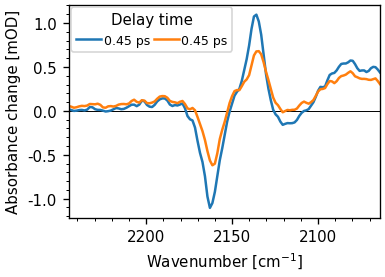
One method to check if the polarization is correct is to plot 1D-spectra at a early delay. The parallel spectrum should have a stronger signal. The following plot shows the 1D-spectra at 0.5 ps delay.

ds_all['para'].integrate_pump().plot.spec(0.5, add_legend=True)
ds_all['perp'].integrate_pump().plot.spec(0.5, add_legend=True)

[<matplotlib.lines.Line2D object at 0x757d3f941290>]

ds_iso.spec2d = ds_iso.spec2d.astype(np.float16)
ds_iso.save_numpy("2D_example.npz")

ds2 = ds_iso.copy()
ds2.spec2d = ds_iso.spec2d.astype(np.float16)

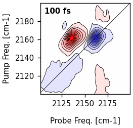
ds2.select_range((2100, 2200), (2100, 2200)).plot.contour(0.1)
ds_iso.select_range((2100, 2200), (2100, 2200)).plot.contour(0.1)

• 
• 

{'fig': <Figure size 315.527x306 with 1 Axes>, 'axs': array([<Axes: >], dtype=object), 0: {'ax': <Axes: >, 'contourf': <matplotlib.contour.QuadContourSet object at 0x757d3f8bf390>, 'contour': <matplotlib.contour.QuadContourSet object at 0x757d43cac5d0>, 'diag_line': <matplotlib.lines.AxLine object at 0x757d3f961250>, 'title': Text(0.05, 0.95, '100 fs')}}