Measuring the system response in the mid IR

In the mid-IR the system response is measured by monitoring the transmittance of the probe light through a thin semi-conductor. skultrafast has an helper function to analyze such a signal.

from skultrafast import messpy, data_io

fname = data_io.get_example_path('sys_response')
tz_result = messpy.get_t0(fname, display_result=False,
                          t_range=(-2, 0.3),
                          no_slope=False)

Newer version of lmfit have a html representation which is used by ipython, e.g. in the notebook. Hence the line below will display the fit results.

tz_result.fit_result

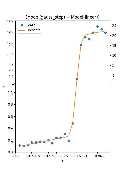
Fit Result

Model: (Model(gauss_step) + Model(linear))

Fit Statistics

fitting method	leastsq
# function evals	37
# data points	22
# variables	5
chi-square	91.2206310
reduced chi-square	5.36591947
Akaike info crit.	41.2892500
Bayesian info crit.	46.7444622
R-squared	0.99752520

Parameters

name	value	standard error	relative error	initial value	min	max	vary	expression
amp	81.9317782	2.48696929	(3.04%)	99.29919985394302	-inf	inf	True
center	-0.51149116	0.00517126	(1.01%)	-0.49999999999999867	-inf	inf	True
sigma	0.07850873	0.00795484	(10.13%)	0.2	-inf	inf	True
slope	6.64703722	1.71198403	(25.76%)	0.0	-inf	inf	True
intercept	69.1447768	2.34423779	(3.39%)	56.77406164675155	-inf	inf	True
FWHM	0.18488807	0.01873366	(10.13%)	0.47100000000000003	-inf	inf	False	sigma*2.355

Correlations (unreported values are < 0.100)

Parameter1	Parameter 2	Correlation
slope	intercept	+0.9610
amp	intercept	-0.9252
amp	slope	-0.8852
amp	sigma	+0.5157
sigma	intercept	-0.4616
sigma	slope	-0.4316
center	intercept	+0.2353
center	slope	+0.1854
amp	center	-0.1036