Comparment Modelling

Here in this tutorial, we will use skultrafast to do global analysis. We are using the approach as presented by van Stokkum (doi:10.1016/j.bbabio.2004.04.01).

The general outline is as follows:

1. Generate a decay associated spectrum

2. Build the transfer matrix K, choosing starting concentrations j

3. Generate transformation matricies from K and j

4. Apply them to the basis vectors of the DAS

Here we assume step 1 is already done. skultrafast has a module to help with step 2. For that we need the Model class. Please note that the module is quite barebones and may still have bugs.

from skultrafast import dataset, data_io, plot_helpers
import numpy as np
from matplotlib import pyplot as plt
from skultrafast.kinetic_model import Model

model = Model()

To build the transfer matrix, we have to add transitions. The if one the compartments is not part of the model it will be added automatically. The following line means that the model has an transition from S2 to S1 with a rate k2. Since no yield is given, it defaults to 1.

model.add_transition('S2', 'S1', 'k2')

Lets also assume, that S1 decays to zero. The comparment zero is special, since it is not modelled explicty and the name zero is reserved.

model.add_transition('S1', 'zero', 'k1')

To get the corresponding matrix from the model we have to call the build_matrix-function

mat = model.build_matrix()
mat

Matrix([
[-k2,   0],
[ k2, -k1]])

To fill the matrix with numeric values we can use the build_matfunc method. This gives us a function which takes all free parameters, first the rates and then the yields.

f = model.build_mat_func()
f

<function _lambdifygenerated at 0x7f985d82cca0>

Now, what can we do with that matrix? We can use it to project the DAS to the described model. For that, we first evaluate the matrix nummerically by supplying values for the parameters

num_mat = f(k2=2, k1=1)
num_mat

array([[-2,  0],
       [ 2, -1]])

Next, we need the eigenvectors of the matrix. Note, that the presented approach assumes that the eigenvalues are simple eigenvalues. If this is not the case, one has to use the jordan normal form. As we see, the eigenvalues of the matrix are the negative rates. That basically means, that the eigenbasis of the problem is given by a diagonal transfer matrix, which is the parallel model described by an DAS. Hence, the eigenvectors allow us to transform the DAS to a SAS and vice versa by using the inverse.

vals, vecs = np.linalg.eig(num_mat)
vals

array([-1., -2.])

To continue, we also need to choose the starting concentrations.

j = np.zeros(len(vals))
j[0] = 1

j

array([1., 0.])

The transformation matrix is then given by

A = vecs @ np.diag(np.linalg.inv(vecs) @ j)
A_inv = np.linalg.inv(A)

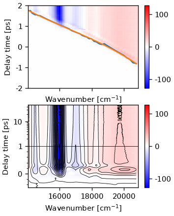
Now DAS @ A_inv should give the SAS, while A_inv @ basis_vecs should return the time-depedence of the concentrations. Let’s test that on some data. Load test data and correct the dispersion.

plot_helpers.enable_style()

wl, t, d = data_io.load_example()
ds = dataset.TimeResSpec(wl, t, d)
dsb = ds.bin_freqs(50)  # Bin dataset to save computation while building docs
res = dsb.estimate_dispersion(heuristic_args=(1.5, ), deg=3, shift_result=.15)

/home/docs/checkouts/readthedocs.org/user_builds/skultrafast/envs/latest/lib/python3.9/site-packages/skultrafast/data_io.py:74: UserWarning: Reading `.npy` or `.npz` file required additional header parsing as it was created on Python 2. Save the file again to speed up loading and avoid this warning.
  wl, data, t = a['wl'], a['data'], a['t']

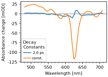
Fit the DAS first.

ids = res.correct_ds
fr = ids.fit_exp([0.0, 0.08, 1, 500000],
                 model_coh=True, fix_sigma=False, fix_t0=False)
ids.plot.das()

[<matplotlib.lines.Line2D object at 0x7f985d2c4c40>, <matplotlib.lines.Line2D object at 0x7f985d2c4160>]

Make sequential Model

m = Model()
m.add_transition('S1hot', 'S1', 'k1')
m.add_transition('S1', 'zero', 'const')
m.build_matrix()

Matrix([
[-k1,      0],
[ k1, -const]])

Make transformation matricies. Notice that we reverse the order of the eigenvectors. Initally, they are sorted by they eigenvalue, therefore the slowest componet comes first. Since this order is inverse of the skultrafast order, we reserve it so we don’t have to reverse our spectra and basis vectors later.

func = m.build_mat_func()
num_mat = func(1 / fr.lmfit_res.params['t0'],
               1/fr.lmfit_res.params['t1'])
vals, vecs = np.linalg.eig(num_mat)

# Reverse order
vecs = vecs[:, ::-1]

j = np.zeros(len(vals))
j[0] = 1

A = (vecs @ np.diag(np.linalg.inv(vecs) @ j)).T
A_inv = np.linalg.inv(A)

The DAS are members of the fitter object. Since we are also modeling coherent contributions, we only take the first two components. Also, the eigenvalue routine sorts the eigenvectors after their eigenvalue, which is the opposite of our usal sorting, where the fast component comes first. T

fig, ax = plt.subplots(2, figsize=(3, 4))

das = fr.fitter.c[:, :2]
ax[0].plot(dsb.wn, das)
ax[0].set_title('DAS')
plot_helpers.lbl_spec(ax[0])

sas = A_inv @ das.T
edas = np.cumsum(das, axis=1)
ax[1].plot(dsb.wn, sas.T)
ax[1].set_title('SAS')
plot_helpers.lbl_spec(ax[1])

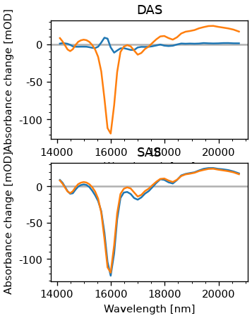
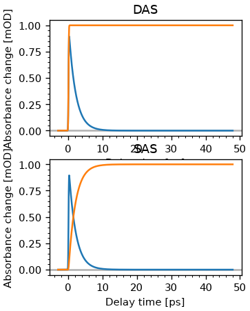
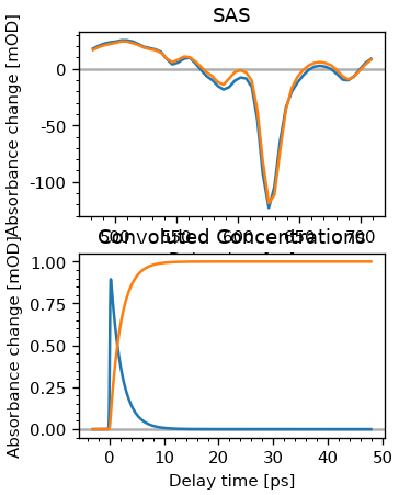
As we can see, we sucessfully get the SAS, which in this case are just EDAS. Let’s also look at the concentrations.

fig, ax = plt.subplots(2, figsize=(3, 4))
ax[0].plot(dsb.t, fr.fitter.x_vec[:, :2])
ax[0].set_title('DAS')
plot_helpers.lbl_trans(ax[0], use_symlog=False)
ct = fr.fitter.x_vec[:, :2] @ A
ax[1].plot(dsb.t, ct)
ax[1].set_title('SAS')
plot_helpers.lbl_trans(ax[1], use_symlog=False)

So why does it work? The dataset is given by the outer product of the concentrations and the spectrum

C = fr.fitter.x_vec[:, :2]
S = das[:, :2]

fit = C @ S.T
fit - fr.fitter.model

array([[-1.86300194e-251, -2.13415894e-251, -1.63260736e-251, ...,
        -5.05015273e-252, -1.86458257e-251, -7.90106447e-252],
       [-7.64672552e-245, -8.75901588e-245, -6.69963937e-245, ...,
        -2.07281632e-245, -7.65443913e-245, -3.24325828e-245],
       [-2.56567084e-238, -2.93863874e-238, -2.24740858e-238, ...,
        -6.95471291e-239, -2.56867859e-238, -1.08828161e-238],
       ...,
       [ 0.00000000e+000,  0.00000000e+000,  0.00000000e+000, ...,
         0.00000000e+000,  0.00000000e+000,  0.00000000e+000],
       [ 0.00000000e+000,  0.00000000e+000,  0.00000000e+000, ...,
         0.00000000e+000,  0.00000000e+000,  0.00000000e+000],
       [ 0.00000000e+000,  0.00000000e+000,  0.00000000e+000, ...,
         0.00000000e+000,  0.00000000e+000,  0.00000000e+000]])

Now we can insert 1 = A @ A_inv. As expected this does not change the product.

((C@A) @ (A_inv @ S.T)) - (C @ S.T)

array([[ 0.00000000e+00,  0.00000000e+00,  0.00000000e+00, ...,
         0.00000000e+00,  0.00000000e+00,  0.00000000e+00],
       [ 0.00000000e+00,  0.00000000e+00,  0.00000000e+00, ...,
         0.00000000e+00,  0.00000000e+00,  0.00000000e+00],
       [ 0.00000000e+00,  0.00000000e+00,  0.00000000e+00, ...,
         0.00000000e+00,  0.00000000e+00,  0.00000000e+00],
       ...,
       [ 0.00000000e+00,  3.55271368e-15,  3.55271368e-15, ...,
         0.00000000e+00,  0.00000000e+00,  0.00000000e+00],
       [ 0.00000000e+00,  3.55271368e-15,  3.55271368e-15, ...,
        -2.22044605e-16,  0.00000000e+00,  1.77635684e-15],
       [ 0.00000000e+00,  0.00000000e+00,  0.00000000e+00, ...,
         0.00000000e+00,  0.00000000e+00,  0.00000000e+00]])

All steps above are done in the make_sas method of the the fitresult, taking a Model as a parameter. If yields are required, they also have to be supplied.

sas, ct = fr.make_sas(model, {})

fig, ax = plt.subplots(2, figsize=(3, 4))
ax[0].plot(fr.fitter.wl, sas.T)
ax[0].set_title('SAS')
plot_helpers.lbl_trans(ax[0], use_symlog=False)
ct = fr.fitter.x_vec[:, :2] @ A
ax[1].plot(dsb.t, ct)
ax[1].set_title('Convoluted Concentrations')
plot_helpers.lbl_trans(ax[1], use_symlog=False)