Dispersion Handling

It is common to use chirped probe pulses in visible fs-pump-probe spectroscopy. This results in a wavelength depended time-zero, since the different probe wavelength arrive at different times at the sample. The chirp is generally well modeled by a low-order polynomial. Therefore to work with dispersion affected spectra, it is necessary to know to dispersion curve.restr

There are various ways to measure the dispersion directly. Alternatively, one can estimate the dispersion directly form the data. The estimate can used to correct the spectrum directly, or if the dispersion is explicitly part of the fitted model, used as the starting guess.

Estimation of the dispersion from the data

skultrafast can estimate the dispersion by first using a heuristic which estimates the time-zero for each wavelengths. The resulting curve is then fitted with a polynomial using a robust fitting method. The robust method is necessary since the heuristics are error-prone.

Heuristics

skultrafast comes with different heuristics to estimate the time-zero from a single trace. The heuristic functions are located in the zero_finding module. Additionally, user-given heuristics are supported. Working directly with the functions should not be necessary, when using the TimeResSpec class.

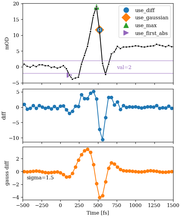
1. use_diff, returns the index where the largest signal change is located.

2. use_max, returns the index with the largest positive signal. This useful when the cross-phase modulation or two-photon contributions are strong, e.g. when measuring solvent signals.

3. use_gaussian, returns the index where the convolution with the first derivative of an gaussian is the largest. This works like a averaged version of use_diff.

4. use_first_abs, returns the earliest index where the absolute of the signal is above a given threshold. The methods works best when the threshold is small, therefore indicating the first signal contributions above the noise floor. This captures the dispersion curve quite well, minus a slight offset, since it captures the beginning of the pump-probe interaction.

The image below compares the results of the different heuristics on a real signal. The signal has strong coherent contributions.

(Source code, svg, png)

The top figure shows a signal and resulting estimates for the different heuristics. The horizontal lines mark the value used by the use_first_abs method. The middle figure shows the difference between sequential points, use_diff just returns the absolute argmax of this differences. The bottom figure shows the convolution with the first derivative of a gaussian with the signal. Again, use_gaussian just returns the absolute argmax of the convolution. The sigma is given in data-points.

Since the signal show strong coherent effects, the use_max method is the method of choice for this trace. But on other wavelengths, the non-coherent signal is stronger and that method may fail. Since both methods based on derivatives differ only by one point and are less suspisusceptible may be the better choice. Looking at the figure, one may be thinking that the use_first_abs heuristic is useless, because it is clearly giving an too early estimatation. But since happens for almost all signals, the heuristic is very useful since it reproduces the (offsetted) dispersion curve quite well.

Robust fitting

In the second step, the resulting \(t_0(\omega)\) data is approximated with a polynomial of low degree, using a robust fitting method form statsmodels. The regression of the time-zeros uses wavenumbers as the depend variable, since the dispersion is proportional to the frequency.

Using the estimate

There are three different ways to use the resulting dispersion curve.

1. Use linear interpolation to correct the dispersion. Here, for every channel we interpolate the data by shift the data-points from (t, y) to (t - disp(wl), y_new).

2. The new values are used to generate binning borders, which are then used to generate the new t-vector.

3. We fit a full model in which the dispersion is explicitly modeled.

For a quick exploration, I recommend the first method. An interpolated dataset is necessary for plotting spectra and maps anyway.