Perturbed free induction decay

Here we shortly derive the perturbed free induction decay using a simple model and implement the analytic solutions. So first, what is the PFID? The PFID is a coherent signal contribution arising in the mid-IR. It manifests as a signal occurring for negative delay times, hence, where the probe arrives before the pump. Naively one would expect an zero signal if the pump arrives before the probe, since the probe can’t possibly interact with pump. But the free induction decay of the vibrations excited by the probe can take picoseconds and can be perturbed by the pump exciting the sample.

This can be shown by a toy-model. The toy-model assumes delta-pulses.

First we do some imports and define a helper plotter function.

import numpy as np
import matplotlib.pyplot as plt
import skultrafast.plot_helpers as ph
import skultrafast.unit_conversions as uc

ph.enable_style()
plt.rcParams['font.size'] = 7

def plot_pulse(ax: plt.Axes, pos: float, color: str, w: float = 0.05):
    new_x = np.linspace(pos - 5*w, pos + 5*w, 100)
    xt = new_x - pos
    y = np.exp(-0.5 * xt**2 / w**2)
    ax.plot(new_x, y, color=color)


def apply_style(axs, label):
    for a in axs:
        a.spines['top'].set_visible(0)
        a.spines['right'].set_visible(0)
        a.set_xlabel(label)
        a.legend(frameon=0, ncol=1)

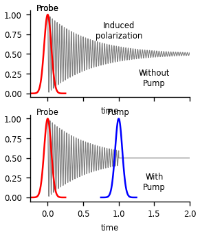
Now lets design our toy model. We simple assume an exponentially decaying polarization and assume the pump destructs the polarization.

fig, (ax, ax2) = plt.subplots(2, 1, figsize=(2.5, 3), sharex='col')

plot_pulse(ax, 0, 'r')
ax.annotate("Probe", xy=(0, 1.05), ha='center')

plot_pulse(ax2, 0, 'r')
plot_pulse(ax2, 1, 'b')
ax2.annotate("Pump", xy=(1, 1.05), ha='center')

for a in [ax, ax2]:
    a.annotate("Probe", xy=(0, 1.05), ha='center')
    a.spines['top'].set_visible(0)
    a.spines['right'].set_visible(0)
    a.set_xlabel('time')

# FID decay and frequency
ts = np.linspace(0, 6, 20000)
T2 = 0.6
T_pump = 1
om = uc.cm2THz(1000)
y1 = np.exp(-ts / T2) * np.cos(om * ts * 2 * np.pi)
yo = y1.copy()
y1[ts > T_pump] = 0

ax.plot(ts, (yo+1) / 2, scalex=0, lw=0.7, c='0.5', zorder=1)
ax.annotate("Induced\npolarization", (1, 0.7), ha='center')
ax.set_xlim(-.25, 2)
ax2.plot(ts, (y1+1) / 2, scalex=0, lw=0.7, c='0.5', zorder=1)
ax.annotate("Without\nPump", (1.5, 0.1), ha='center')
ax2.annotate("With\nPump", (1.5, 0.1), ha='center')

Text(1.5, 0.1, 'With\nPump')

The upper plot shows the FID of the polarization in the sample. The bottom plot show hows the FID could be perturbed by the pump. In this example, the pump leads to destruction of the polarization. Next, we will simulate the resulting spectra for both shown cases. For that, we calculate the Fourier-transform of each polarization and take the real parts.

fig, (ax, ax2) = plt.subplots(2, 1, figsize=(2.5, 3), sharex='col')

freqs = np.fft.rfftfreq(yo.size * 2, ts[1] - ts[0])
freqs_cm = uc.THz2cm(freqs)
sp1 = np.fft.rfft(yo, n=yo.size * 2).real
ax.plot(freqs_cm, sp1, label='FID', c='r')
ax.set_xlim(900, 1100)

sp2 = np.fft.rfft(y1, y1.size * 2).real
ax.plot(freqs_cm, sp2, label='PFID (t=1 ps)', c='b')
ax2.plot(freqs_cm, sp2 - sp1, c='xkcd:blood', label='Difference')
apply_style([ax, ax2], 'time')

/home/docs/checkouts/readthedocs.org/user_builds/skultrafast/envs/latest/lib/python3.9/site-packages/skultrafast/unit_conversions.py:92: RuntimeWarning: divide by zero encountered in divide
  return cm2fs(1e3 / THz)

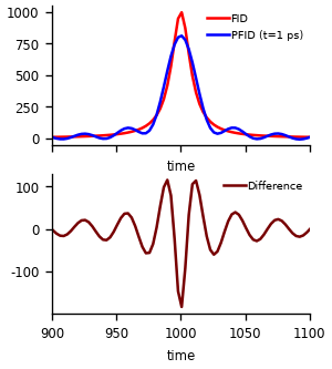
The upper figure shows the resulting spectra. As expected, the FID decay results in a Lorentzian line shape, while the PFID show additional oscillations. It is important to realize that the PFID signal is depended on time delay between pump and probe. The shown spectra is calculated for delay of 1 ps and an $T_2$ duration of 0.6 ps. The frequency was chosen to be equal to 1000 cm-1.

In the experiment, we compare the spectra with and without pump. Hence, the recorded signal, shown in the bottom figure, is the difference of the two spectra.

So far, we assumed that the perturbation due to the pump leads to destruction of the polarization. This should be a rare case for real in real systems. In most cases, the interaction of with the pump will leads to a frequency shift, either by promoting the molecule to an electronically excited state (visible pump) or to an higher vibrational state (IR pump). In our toy model, this can be modeled by switching the frequency at 1 ps. Here we assume no phase change.

fig, ax = plt.subplots(1, 1, figsize=(2.5, 2), sharex='col')

# FID decay and frequency
# Same as above
om2 = uc.cm2THz(1000-15)  # Assuming 15 cm-1 red shift


y2 = np.exp(-ts / T2) * np.cos(om*ts*2*np.pi)
dphi = om2*T_pump - om*T_pump  # Phase correction
yt = np.exp(-ts / T2) * np.cos(om2*(ts-T_pump)*2*np.pi)

ax.set_xlim(-.25, 2)
plot_pulse(ax, 1, color='b')
yo = y2.copy()

y2[ts > T_pump] = yt[ts > T_pump]
ax.plot(ts, (y2+1) / 2, scalex=0, lw=0.5, c='r', zorder=1, label='PFID')
ax.plot(ts, (yo+1) / 2, scalex=0, lw=1.3, c='0.6', zorder=.9, label='FID')
ax.set(xlim=(0.8, 1.5))

ax.legend(frameon=0)
ax.annotate("Pump", xy=(1, 1.05), ha='center')
apply_style([ax], 'freq')

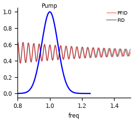
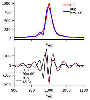
So how does the spectrum look in this case? Remeber that the FT is a linear operation. Hence we could build the spectrum by the sum of the case above and phase and amplitude shifted FID with the shifted frequency. But first let’s take the FT directly

fig, (ax, ax2) = plt.subplots(2, 1, figsize=(2.5, 3), sharex='col')

ax.set_xlim(900, 1100)

sp3 = np.fft.rfft(y2, y2.size * 2).real
ax.plot(freqs_cm, sp1, label='FID', c='r')
ax.plot(freqs_cm, sp3, label='PFID\n(t=1 ps)', c='b')
ax2.plot(freqs_cm, sp2 - sp1, c='xkcd:blood', label='PFID\n(bleach)', lw=1)
ax2.plot(freqs_cm, sp3 - sp1, c='xkcd:navy', label='PFID\n(shift)', lw=1)
apply_style([ax, ax2], 'freq')

Let check the assumption above.

fig, ax = plt.subplots(1, 1, figsize=(2.5, 2), sharex='col')

y3 = y2.copy()
y3[ts<T_pump] = 0

ax.plot(ts, (y3+1) / 2, scalex=1, lw=0.5, c='r', zorder=1, label='PFID')
ax.plot(ts, (y1+1) / 2 + .7, scalex=1, lw=0.5, c='b', zorder=1, label='PFID')
ax.plot(ts, (y1+y3) / 2 - .3, scalex=1, lw=0.5, c='xkcd:green', zorder=1, label='PFID')

ax.text(1, 0.9, '+', fontsize=12)
ax.text(1, 0, '=', fontsize=12)
ax.set(xlim=(0, 2))
for a in [ax, ]:
    a.spines['top'].set_visible(0)
    a.spines['right'].set_visible(0)

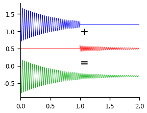
Indeed, the sum of these is equal to our freq jump.

print(np.allclose(y1+y3, y2))

True

We know already how the specturm of the blue polarization looks like, but how looks spectrum of the red part? It is not just a pure FID with the new frequency, since the initial phase depends on the time-delay between pump and probe.

In the figure below we show that the sum of spectra of the separate parts has the same spectra as the sum. As mentioned, this is expected since the FT is linear. In bottom we see, that we get the same result as in the figure above.

fig, (ax, ax2) = plt.subplots(2, 1, figsize=(2.5, 3), sharex='col')

ax.set_xlim(900, 1100)

sp4 = np.fft.rfft(y3, y2.size * 2).real

ax.plot(freqs_cm, sp1, lw=1, label='1 FID', c='r')
ax.plot(freqs_cm, sp2, lw=1, label='2 PFID\n(bleach)', c='b')
ax.plot(freqs_cm, sp3, lw=1, label='3 PFID\n(freq shift)', c='xkcd:orange')
ax.plot(freqs_cm, sp4, lw=1, label='4 PFID\n(new freq only)', c='xkcd:green')
ax2.plot(freqs_cm, sp2 - sp1, c='b', label='2-1', lw=1)
ax2.plot(freqs_cm, sp3 - sp1, c='xkcd:orange', label='3-1', lw=2)
ax2.plot(freqs_cm, sp4  + sp2 - sp1, c='xkcd:green', label='2+4-1', lw=1)

apply_style([ax, ax2], 'freq')

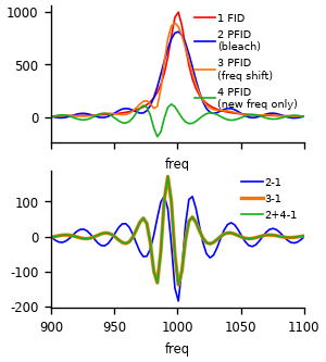
Note that this implies that a pump-induced phase change also gives rise to PFID. Let’s simulate the spectrum for that case. Note that the used phase jumps are exaggerated for common cases. But for excitation of vibronic progression, such jump may be happing.

fig, (ax, ax2) = plt.subplots(2, 1, figsize=(2.5, 3), sharex='col')

ax.set_xlim(900, 1100)

y4 = np.exp(-ts / T2) * np.cos(om*ts*2*np.pi)
djump = np.pi # Phase jump
yt = np.exp(-ts / T2) * np.cos(om*ts*2*np.pi - djump)
y4[ts>T_pump] = yt[ts>T_pump]
sp5 = np.fft.rfft(y4, y2.size * 2).real

y5 = np.exp(-ts / T2) * np.cos(om*ts*2*np.pi)
djump = np.pi/2 # Phase jump
yt = np.exp(-ts / T2) * np.cos(om*ts*2*np.pi - djump)
y5[ts>T_pump] = yt[ts>T_pump]
sp6 = np.fft.rfft(y5, y2.size * 2).real

y6 = np.exp(-ts / T2) * np.cos(om*ts*2*np.pi)
djump = np.pi*0.1 # Phase jump
yt = np.exp(-ts / T2) * np.cos(om*ts*2*np.pi - djump)
y6[ts>T_pump] = yt[ts>T_pump]
sp7 = np.fft.rfft(y6, y2.size * 2).real

ax.plot(freqs_cm, sp1, lw=1, label='1 FID', c='r')
ax.plot(freqs_cm, sp2, lw=1, label='2 PFID\n  (bleach)', c='b')
ax.plot(freqs_cm, sp5, lw=1, label='3 $\\pi$', c='c')
ax.plot(freqs_cm, sp6, lw=1, label='4 $\\pi/2$ ', c='xkcd:grey')
ax.plot(freqs_cm, sp7, lw=1, label='5 $\\pi/10$', c='xkcd:violet')

ax2.plot(freqs_cm, sp2 - sp1, c='b', label='2-1', lw=1)
ax2.plot(freqs_cm, sp5 - sp1, c='xkcd:orange', label='3-1', lw=1)
ax2.plot(freqs_cm, sp6 - sp1, c='xkcd:grey', label='4-1', lw=1)
ax2.plot(freqs_cm, sp7-sp1, lw=1, label='5-1', c='xkcd:violet')

apply_style([ax, ax2], "freq")

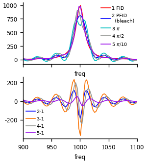
It is interesting to see, that the effect of the phase distortion can be larger than the effect of full bleaching.

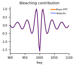
Comparision to analytic expressions

Of course there are also analytic expressions for the PFID. Afaik, these expression assume zero phase change due to the pump interaction. According to the literature, setting \(\Delta\omega = \omega - \omega_{10}\\\), the bleaching contribution is given by

\[S^{(R_4)}_{PFID}(T, \omega) \propto e^{-T/T_2}\frac{(1/T_2) \cos[\Delta\omega T]-\Delta\omega\sin[\Delta\omega T]}{(\Delta\omega)^2+(1/T_2)^2}\]

For the excited state absorbtion, we additionally use \(\Delta\omega_{21} = \omega - \omega_{21}\\\) and get

\[S^{(R_6)}_{PFID}(T, \omega) \propto e^{-T/T_2}\frac{(1/T_2) \cos[\Delta\omega T]-\Delta\omega\sin[\Delta\omega_{21} T]}{(\Delta\omega_{21})^2+(1/T_2)^2}\]

This can be directly translated into code: Note that the implementations of these two functions can be found in skultrafast.utils

def pfid_r4(T, om, om_10, T_2):
    om = uc.cm2THz(om)*2*np.pi
    om_10 = uc.cm2THz(om_10)*2*np.pi
    dom = om - om_10
    num = (1/T_2)*np.cos(dom*T)-dom*np.sin(dom*T)
    return np.exp(-T/T_2)*num/(dom**2+(1/T_2**2))

def pfid_r6(T, om, om_10, om_21, T_2):
    om = uc.cm2THz(om)*2*np.pi
    om_10 = uc.cm2THz(om_10)*2*np.pi
    om_21 = uc.cm2THz(om_21)*2*np.pi
    dom = om - om_10
    dom2 = om - om_21
    num = (1/T_2)*np.cos(dom*T)-dom2*np.sin(dom*T)
    return np.exp(-T/T_2)*num/(dom2**2+(1/T_2**2))

#  %%
#  Now we compare the analytic solution with our previous results

fig, ax= plt.subplots(1, 1, figsize=(2.5, 2), sharex='col')

y_ana = pfid_r4(1, freqs_cm, 1000, 0.6)

ax.set(xlim=(900, 1100), title='Bleaching contribution')
ax.plot(freqs_cm, (sp2-sp1)/(sp2-sp1).max(), lw=2, color='xkcd:orange', label='From FFT')
ax.plot(freqs_cm, y_ana/y_ana.min(), label='Analytic', lw=1, color='b')
apply_style([ax], "freq")

/home/docs/checkouts/readthedocs.org/user_builds/skultrafast/envs/latest/lib/python3.9/site-packages/skultrafast/unit_conversions.py:31: RuntimeWarning: divide by zero encountered in divide
  return 1 / (t*1e-15*c_cm)

As we can see, the signals are indeed identical. Let’s see if the same is true for the excited state contribution. The analytical solution should be identical to our shift-only spectrum.

fig, ax = plt.subplots(1, 1, figsize=(2.5, 2), sharex='col')

y_ana = pfid_r6(1, freqs_cm, 1000, 1000-15, 0.6)

ax.set(xlim=(900, 1100))
ax.plot(freqs_cm, (sp4/sp4.max()), lw=2, color='xkcd:orange', label='From FFT')
ax.plot(freqs_cm, y_ana/y_ana.max(), label='Analytic', lw=1, color='b')
ax.set_title('Excited-state contribution')

apply_style([ax], "freq")

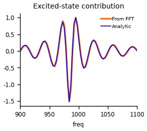
As we can see, the signals are indeed identical! Hence our toy-model is just a different representation. Still, the simple model reveals a shortcomming in the approach used to derive the analytic expressions: it assumes no phase-change upon pump interaction, which is not true for all systems.