Starting tutorial

First we import numpy, matplotlib and skultrafast. For reproducebilty we should always print out the version of skultrafast

import matplotlib.pyplot as plt
from skultrafast.dataset import TimeResSpec
from skultrafast import plot_helpers
import skultrafast
from skultrafast import data_io
skultrafast.__version__

'0+untagged.69.g25010a7'

Some matplotlib setting for nicer pictures.

plt.rcParams['figure.dpi'] = 150
plt.rcParams['figure.figsize'] = (4, 3)
plt.rcParams['figure.autolayout'] = True
plt.rcParams['font.size'] = 9

Creating a TimeResSpec

In this tuturial we use the example data which is provided by skultrafast. The load_example function gives us three arrays. One containing the wavelengths, another one containing the delay times and one two dimensional array containing the data in mOD.

wavelengths, t_ps, data_mOD = data_io.load_example()

/home/docs/checkouts/readthedocs.org/user_builds/skultrafast/envs/latest/lib/python3.9/site-packages/skultrafast/data_io.py:74: UserWarning: Reading `.npy` or `.npz` file required additional header parsing as it was created on Python 2. Save the file again to speed up loading and avoid this warning.
  wl, data, t = a['wl'], a['data'], a['t']

Lets look at the constructor of the TimeResSpec (Time resolved Spectra) class, which is the main object when working with single data:

print(TimeResSpec.__init__.__doc__)

Class for working with time-resolved spectra. If offers methods for
analyzing and pre-processing the data. To visualize the data,
each `TimeResSpec` object has an instance of an `DataSetPlotter` object
accessible under `plot`.

Parameters
----------
wl : array of shape(n)
    Array of the spectral dimension
t : array of shape(m)
    Array with the delay times.
data : array of shape(n, m)
    Array with the data for each point.
err : array of shape(n, m) or None (optional)
    Contains the std err of the data, can be `None`.
name : str (optional)
    Identifier for data set.
freq_unit : 'nm' or 'cm' (optional)
    Unit of the wavelength array, default is 'nm'.
disp_freq_unit : 'nm','cm' or None (optional)
    Unit which is used by default for plotting, masking and cutting
    the dataset. If `None`, it defaults to `freq_unit`.

Attributes
----------
wavelengths, wavenumbers, t, data : ndarray
    Arrays with the data itself.
plot : TimeResSpecPlotter
    Helper class which can plot the dataset using `matplotlib`.
t_idx : function
    Helper function to find the nearest index in t for a given time.
wl_idx : function
    Helper function to search for the nearest wavelength index for a
    given wavelength.
wn_idx : function
    Helper function to search for the nearest wavelength index for a
    given wavelength.

auto_plot : bool
    When True, some function will display their result automatically.

As we see, we can supply all the required parameters. Since the freq_unit defaults to ‘nm’ we don’t need to supply this argument.

ds = TimeResSpec(wavelengths, t_ps, data_mOD)

The TimeResSpec object simply consists of data itself and methods using that data. The attributes containing the data can be accessed under ds.data, ds.wavenumbers, ds.wavelengths and ds.t.

print(ds.data.shape, ds.t.shape, ds.wavelengths.shape)

(409, 800) (409,) (800,)

The TimeResSpec object also has some helper methods to work with the data. These functions find the index of the nearest value for a given number, e.g. to find the position in the time array where the time is zero we can call the t_idx method

print(ds.t_idx(0), ds.t[ds.t_idx(0)])

75 0.0

Hence the spectrum at t = 0 is given by

y_0 = ds.data[ds.t_idx(0), :];

In addition, there is also a shorthand to return the data at these indices directly.

assert(sum(ds.t_d(0) - y_0) == 0)

Overview map

To get an general idea of the transient spectra we need to see it. All plotting functions are in the TimeResSpec.plot object, which is an instance of TimeResSpecPlotter. The plotting functions are using the disp_freq_unit of the dataset as frequency scale by default. This can be changed by changing the disp_freq_unit of the TimeResSpecPlotter object.

ds.plot.disp_freq_unit = 'nm'  # does nothing, since 'nm' is the default
# ds.plot.disp_freq_unit = 'cm' would use wavenumbers

First, we want to check if the dataset is corrected for dispersion. For that we plot a colormap around the time-zero.

ds.plot.map(symlog=0, con_step=10., con_filter=(3, 10))
plt.ylim(-2, 2)

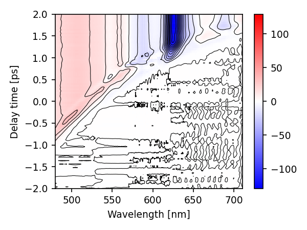
(-2.0, 2.0)

Evidently, the dataset is not corrected for dispersion. Since it is easier to work with a dispersion corrected dataset, we try to estimate the dispersion using the data directly.

Dispersion estimation and correction

skultrafast does this by first using a simple heuristic for determining the time- zero for each transient. The resulting dispersion curve is then fitted with a poly- nominal, using a robust fitting method. More details are given in the documentation.

To estimate the dispersion just call the function. It will plot two colormaps, one with the original dataset, the time-zeros found by the heuristic and the robust polynomial fit of these values. The bottom color map shows the dispersion corrected data.

res = ds.estimate_dispersion(heuristic_args=(1.5,), deg=3)

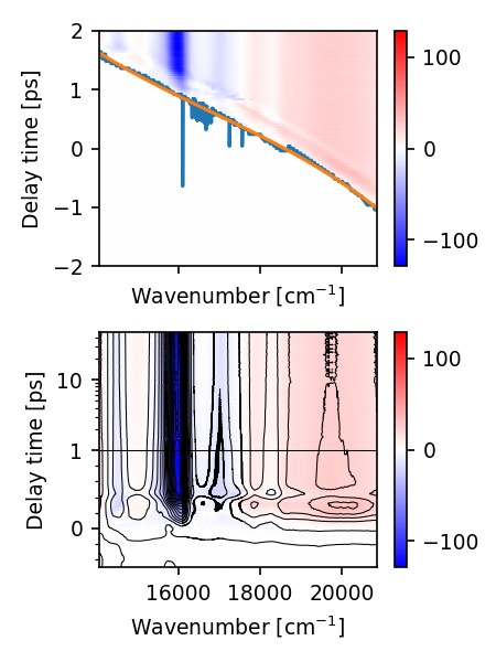
By default, skultrafast uses a very simple heuristic to find the time-zero. It looks for the earliest value above a given limit in each transient, and therefore underestimates the time-zero systematically. Therefore we slightly shift the time-zero.

This generally works surprisingly well. But if the exact time-zero is necessary, I recommend to try other methods or measure the dispersion directly.

WARNING: The cell below changes the dataset inplace. Therefore repeated calls to the cell will shift the time-zero again and again. The shifting can also be applied setting the shift_result parameter in the call to ds.estimate_dispersio.

new_ds = res.correct_ds  # Warning, this does not copy the dataset!
new_ds.t -= 0.2

Plotting spectra and transients

A major part of skultrafast are convenience functions for generating figures. Starting with the colormap from above, we see now that our dataset looks correct:

new_ds.plot.map(con_step=10., con_filter=(3, 5))

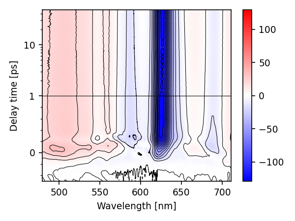
(<matplotlib.collections.QuadMesh object at 0x7f9860ab80d0>, <matplotlib.contour.QuadContourSet object at 0x7f985e85fbe0>)

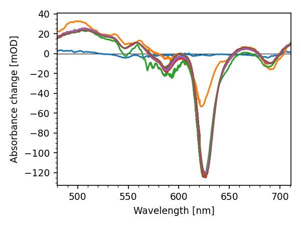
To plot spectra at given delay times:

lines = res.correct_ds.plot.spec(-.2, 0.05, 0.3, 1, 2, 150)

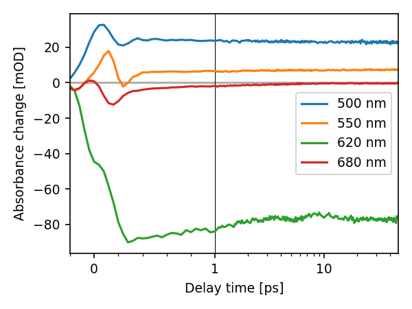
Or plot transients for given wavelengths:

lines = res.correct_ds.plot.trans(500, 550, 620, 680)

All these function offer a number of options. More information can be found in their docstrings.

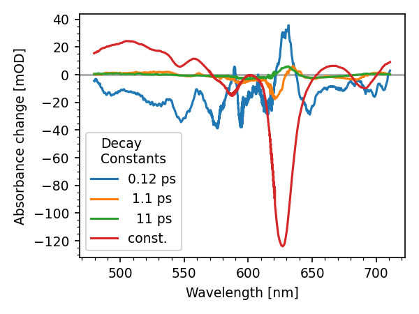
Exponential fitting

Fitting a decay-associated spectra (DAS) is a one-liner in skultrafast. If the dataset is dispersion corrected, only a starting guess is necessary. Please look at the docstring to see how the starting guess is structured. _Note_, the the fitting interface may change in the future.

fit_res = new_ds.fit_exp([-0.0, 0.05, 0.2, 2, 20, 10000],
                          model_coh=True, fix_sigma=False, fix_t0=False)
fit_res.lmfit_res.params

/home/docs/checkouts/readthedocs.org/user_builds/skultrafast/envs/latest/lib/python3.9/site-packages/numba/core/typed_passes.py:336: NumbaPerformanceWarning:
The keyword argument 'parallel=True' was specified but no transformation for parallel execution was possible.

To find out why, try turning on parallel diagnostics, see https://numba.readthedocs.io/en/stable/user/parallel.html#diagnostics for help.

File "../../../../envs/latest/lib/python3.9/site-packages/skultrafast/base_funcs/base_functions_numba.py", line 62:
@njit(parallel=True, fastmath=True, cache=True)
def _fold_exp_and_coh(t_arr, w, tz, tau_arr):
^

  warnings.warn(errors.NumbaPerformanceWarning(msg,

Parameters

name	value	standard error	relative error	initial value	min	max	vary
p0	0.03914888	2.6249e-04	(0.67%)	-0.0	-inf	inf	True
w	0.12264944	1.0606e-04	(0.09%)	0.05	0.00000000	inf	True
t0	0.12332615	7.8396e-04	(0.64%)	0.2	0.10000000	inf	True
t1	1.11185259	0.00597462	(0.54%)	2	0.10000000	inf	True
t2	10.8926809	0.09901834	(0.91%)	20	0.10000000	inf	True
t3	10000.0000	0.00000000	(0.00%)	10000	0.10000000	inf	False

Lets plot the DAS

new_ds.plot.das()

[<matplotlib.lines.Line2D object at 0x7f985d4a3940>, <matplotlib.lines.Line2D object at 0x7f985d4a39a0>, <matplotlib.lines.Line2D object at 0x7f985d4a3670>, <matplotlib.lines.Line2D object at 0x7f985d4a3e80>]

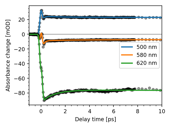
We can always work with the results directly to make plots manually. Here, the t_idx, wl_idx and wn_idx methods of the dataset are very useful:

for wl in [500, 580, 620]:
    t0 = fit_res.lmfit_res.params['p0'].value
    idx = new_ds.wl_idx(wl)
    plt.plot(new_ds.t - t0, fit_res.fitter.data[:, idx], 'o', color='k', ms=4,
             alpha=0.4)
    plt.plot(new_ds.t - t0, fit_res.fitter.model[:, idx], lw=2, label='%d nm' % wl)
plt.xlim(-1, 10)
plot_helpers.lbl_trans(use_symlog=False)
plt.legend(loc='best', ncol=1)

<matplotlib.legend.Legend object at 0x7f985d639a60>