Spectrograph calibration

In this tutorial we look at the calibration of an spectrograph. So what we looking for is a function which is mapping the index of our detector element to a wavelength.

We discuss two cases:

1. The spectrograph grating is fixed.

2. The spectrograph grating is rotateable.

For the first case, we need to have serveral identifiable feautres with known spectral positions. The can be a calibration pen lamp (ideal), a sample with known absorption peaks or known filters. The calibration than is done by fitting the result index vs. wavelength points with a function. For a typical grating spectrometer the function should be a linear function. Depending on the imaging geometry, a higher polynomial can be used.

For the second case, we can get away with one known feature. For this, we must assume that grating information and stepper settings are correct, e.g. the spectrograph moves the grating the correct distancance. This can be checked by first adjusting the zero-oder correctly and then moving the grating to a known peak. The peak-postion should then coindcide with the zero-order postion. If the zero-order can not be aligned, it may be that the zero-offsets of the spectrograph are incorrect. These can often be modified, the easies way is to use the software of the spectrograph. We then record the spectrum by scanning the feature in a way, that it moves from one side of the detector to the other. Now by comparing the wavelength which has been set to feature position, we can directly see the dispersion per pixel. This, again, should be linear for most spectrographs.

Notice that tracking a feature over the whole range manually is not efficent, if possible it should be automated, e.g. by always looking for the lowest intensity.

Lets look at an example. Here, we are looking at the calibartion of an 128 channels spectrometer in the mid-IR.

Imports we will use later.

import numpy as np
import matplotlib.pyplot as plt
import scipy.ndimage as nd
from scipy.stats import linregress
from skultrafast import data_io

Nicer plots.

from skultrafast.plot_helpers import enable_style
enable_style()

The file contains the measured intensities of the recored lines, the set wavelength and the calculated wavelengths, which we want to check and adjust.

p = data_io.get_example_path('ir_polyfilm')
a = np.load(p)
list(a.keys())

['probe', 'wl']

Use some helper variables

wl = a['wl']
N = 63  # center channel
cwl = a['wl'][:, N]
pr = a['probe']

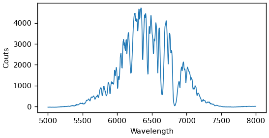
Lets plot the spectrum of the center channel.

fig, ax = plt.subplots(figsize=(5, 2.4))
ax.plot(cwl, pr[:, 64], lw=1)
#ax.secondary_xaxis('top', functions=(lambda x: 1e7 / x, lambda x: 1e7 / x))
plt.setp(ax, xlabel='Wavelength', ylabel='Couts')

[Text(0.5, 41.00000000000002, 'Wavelength'), Text(40.99999999999998, 0.5, 'Couts')]

The spectrum consists of the probe, with absorption lines showing up as dips. The sharp lines are caused by water-vapor and the wider lines are from a polystyrene calibration film.

To extract the real absorption spectrum we can measure the spectrum without the film and calculate the absorption. It is also possible to subtract the baseline. This approach also allows us to use water-vapor lines for calibration. Notice that latter also depend on the humidity and temperature, also the presented baseline approach is just an approximation.

We approximate the baseline by taking the local maxima and interpolate inbetween.

from scipy.interpolate import interp1d
for ch in [63, 58]:
    fig, ax = plt.subplots()
    back = nd.maximum_filter1d(pr[:, ch], 15)
    idx = back == pr[:, ch]

    idx[:200] = False
    idx[-100:] = False
    touching = back[idx]
    f = interp1d(cwl[idx], touching, bounds_error=False, kind='cubic')
    plt.plot(cwl, f(cwl))
    plt.plot(cwl, pr[:, ch])
    plt.plot(cwl, np.interp(cwl, cwl[idx], touching) - pr[:, ch] + 5000, lw=1)

    # Load water vapor data
    p = data_io.get_example_path('vapor')
    ftir_x, ftir_vapor= np.load(p).T

    # Convolve vapor spectrum with a gaussian
    ftir_vapor = nd.gaussian_filter(ftir_vapor, 5) * 52000

    ax.plot(1e7 / ftir_x, ftir_vapor + 5000, scaley=0, lw=1, zorder=1, alpha=0.5, label='Water Vapor')
    plt.plot(cwl, pr[:, ch] + np.interp(cwl, 1e7 / ftir_x, ftir_vapor), lw=2, color='C5')
    ax.axhline(5000, lw=1, c='0.3')

    ax.vlines(1e7 / np.array([1493, 1452, 1601]),
              5000,
              8000,
              color='C4',
              zorder=3,
              label='Polysteren peak pos.')

    ax.set(xlim=(6000, 7000),
           ylim=(0, 10000),
           xlabel='Wavelenght / nm',
           title=f'Channel: {ch}')
    ax.legend(ncol=4)
    #ax.secondary_xaxis('top', functions=(lambda x: 1e7 / x, lambda x: 1e7 / x))

• 
• 

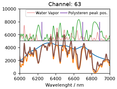
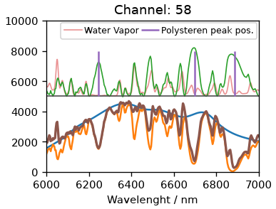
Using the initial channel 63 clearly leads to an offset, indicating the zero-order position was not correct. Using instead 58 as the center channel we get an good agreement. The peak at 1601 is isolated from water vapor lines, hence we will use it to calibrate the dispersion. For that we will look at three spectra at once: One where the peak is at the center channel and one for each side. We will try to find a suitable dispersion factor to get some reasonable overlap. As seen below, a factor of 7.7 nm/pixel gives us really good fit.

fig, ax = plt.subplots()
i = np.argmin(abs(cwl - 1e7/1601))
disp = 7.7
new_x = disp * (np.arange(128) - 58)
ax.plot(new_x + cwl[i], pr[i, :])
ax.plot(new_x + cwl[i - 130], 0.58 * pr[i - 130, :])
ax.plot(new_x + cwl[i + 130], 1.4 * pr[i + 130, :])

new_wl = disp * (np.arange(128) - 58)[:, None] + cwl[None, :]

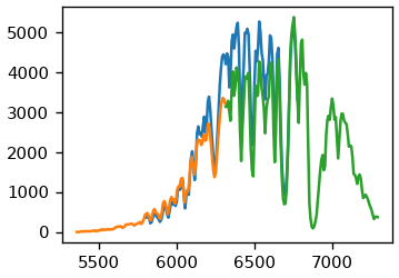
Using that factor we can extract the region around the peak for multiple spectra. In this region, we just look for the minimum.

fig, (ax, ax2) = plt.subplots(2, sharex=True, figsize=(3, 4))

mask = (abs(new_wl - 1e7/1601) < 80).T
ax.plot(np.arange(128) - 58, cwl[np.argmax(mask, 0)], lw=1, c='k', ls='--')
ax.plot(np.arange(128) - 58, cwl[800 - np.argmax(mask[::-1], 0)], lw=1, c='k', ls='--')
ax.pcolormesh(np.arange(128) - 58, cwl, pr, rasterized=True, shading='auto')

tmp = np.where(mask, pr, np.inf)
from scipy.stats import linregress

x = np.arange(128) - 58
y = cwl[np.argmin(tmp, 0)]
res

Traceback (most recent call last):
  File "/home/docs/checkouts/readthedocs.org/user_builds/skultrafast/checkouts/latest/skultrafast/examples/tutorial_spectrometer_calibration.py", line 169, in <module>
    res
NameError: name 'res' is not defined