Note
Go to the end to download the full example code.
Messpy v1 Example
This example shows how to load files from MessPy v1, hence it is only of interested for people working with files produced by it. Here we loading a datafile, which used our infrared detection setup.
MessPy v1 files are .npz files, which consists of zipped npy (numpy) files. Under the module messpy we a helper class to work with it. We will start with importing the module and the standard tools.
from skultrafast import messpy, dataset, data_io
import matplotlib.pyplot as plt
import skultrafast
print(skultrafast.__version__)

plt.rcParams['figure.dpi'] = 130
plt.rcParams['figure.figsize'] = (3.2, 2)
plt.rcParams['figure.autolayout'] = True
6.0
The main tool is the MessPyFile class. Note the constructor takes all the
neccesary information to do the processing. Here I will pass all parameters
explictily for documentation proposes. Some of the parameters are infered
automatically.
# Get the file location first

fname = data_io.get_example_path('messpy')
print("Tutorial MessPy-file located at %s" % fname)
mpf = messpy.MessPyFile(
    fname,
    invert_data=True,  # Changes the sign of the data
    is_pol_resolved=True,  # If the data was recored polarization resolved.
    pol_first_scan='perp',  # Polarisation of the first scan
    valid_channel=1,  # Which channel to use, recent IR data always uses 1
    # Recent visible data uses 0
)

print(mpf.data.shape)
Tutorial MessPy-file located at /home/docs/checkouts/readthedocs.org/user_builds/skultrafast/envs/latest/lib/python3.11/site-packages/skultrafast/examples/data/messpyv1_data.npz
/home/docs/checkouts/readthedocs.org/user_builds/skultrafast/envs/latest/lib/python3.11/site-packages/skultrafast/messpy.py:174: RuntimeWarning: overflow encountered in cast
  self.wavenumbers = 1e7 / self.wl
(3, 150, 32, 2, 15)
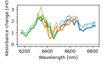
Simlar to TimeResSpec the MessPyFile class has a plotter subclass with various
plot methods. For example, the compare_spec method plots a averaged spectrum
for each central channel recored.
mpf.plot.compare_spec()
/home/docs/checkouts/readthedocs.org/user_builds/skultrafast/envs/latest/lib/python3.11/site-packages/numpy/ma/core.py:4450: RuntimeWarning: overflow encountered in multiply
  self._data.__imul__(other_data)
/home/docs/checkouts/readthedocs.org/user_builds/skultrafast/envs/latest/lib/python3.11/site-packages/skultrafast/dataset.py:174: RuntimeWarning: overflow encountered in cast
  self._wavenumbers = 1e7 / wl
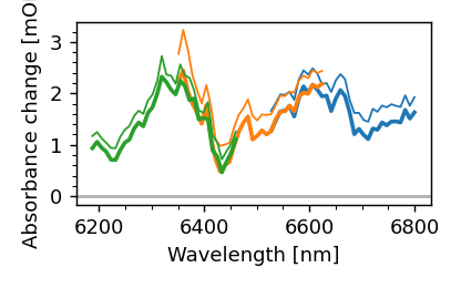
As we can see, the applied wavelength calibration used by messpy was not correct. Let’s change that.
mpf.recalculate_wavelengths(8.8)
mpf.plot.compare_spec()
Note that MessPyFile uses sigma clipping when averaging the scans. If you
want more control over the process, use the average_scans method. For
example here we change the clipping range and use only the first 5 scans.
mpf.average_scans(sigma=2, max_scan=20);
{'para0': <skultrafast.dataset.TimeResSpec object at 0x77f8a29e7d50>, 'perp0': <skultrafast.dataset.TimeResSpec object at 0x77f8a2a90550>, 'iso0': <skultrafast.dataset.TimeResSpec object at 0x77f8a29f3050>, 'para1': <skultrafast.dataset.TimeResSpec object at 0x77f8a2aa3090>, 'perp1': <skultrafast.dataset.TimeResSpec object at 0x77f8a2aa27d0>, 'iso1': <skultrafast.dataset.TimeResSpec object at 0x77f8a29ee210>, 'para2': <skultrafast.dataset.TimeResSpec object at 0x77f8a2ab6090>, 'perp2': <skultrafast.dataset.TimeResSpec object at 0x77f8a2bc8510>, 'iso2': <skultrafast.dataset.TimeResSpec object at 0x77f8a2bc9f90>}
The indivudal datasets, for each polarization and each spectral window can be found in a dict belonging to the class.
for key, ds in mpf.av_scans_.items():
    print(key, ds)
para0 <skultrafast.dataset.TimeResSpec object at 0x77f8a29e7d50>
perp0 <skultrafast.dataset.TimeResSpec object at 0x77f8a2a90550>
iso0 <skultrafast.dataset.TimeResSpec object at 0x77f8a29f3050>
para1 <skultrafast.dataset.TimeResSpec object at 0x77f8a2aa3090>
perp1 <skultrafast.dataset.TimeResSpec object at 0x77f8a2aa27d0>
iso1 <skultrafast.dataset.TimeResSpec object at 0x77f8a29ee210>
para2 <skultrafast.dataset.TimeResSpec object at 0x77f8a2ab6090>
perp2 <skultrafast.dataset.TimeResSpec object at 0x77f8a2bc8510>
iso2 <skultrafast.dataset.TimeResSpec object at 0x77f8a2bc9f90>
Now we can work with them directly. For example datasets can be combined manually
iso_merge = mpf.av_scans_['iso0'].concat_datasets(mpf.av_scans_['iso1'])
all_iso = iso_merge.concat_datasets(mpf.av_scans_['iso2'])
Since this is quite common, this is also automated by the avg_and_concat
method.
para, perp, iso = mpf.avg_and_concat()
iso.plot.spec(1, 3, 10, n_average=5);
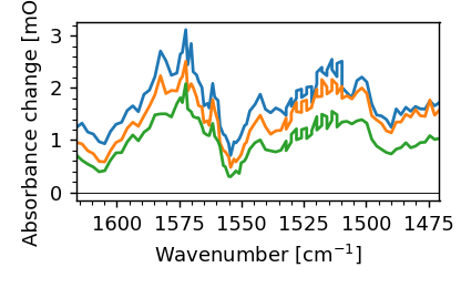
[<matplotlib.lines.Line2D object at 0x77f8a2ab5ad0>, <matplotlib.lines.Line2D object at 0x77f8a2bd5310>, <matplotlib.lines.Line2D object at 0x77f8a2bd6910>]
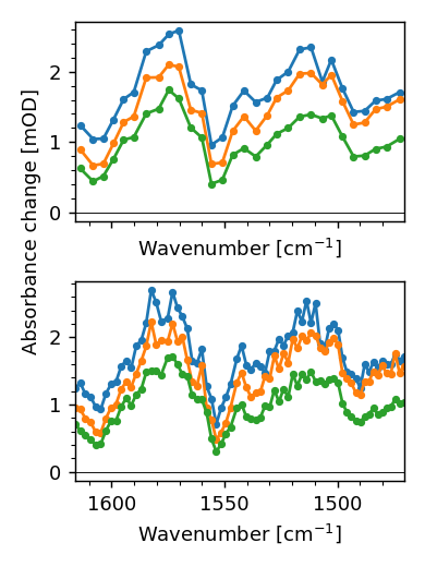
The spectrum looks a little bit janky now, since after merging the datasets the points in the overlapping regions were seperataly recorded and the noise within a recording is correlated. Hence, while the spectrum looks kind of smooth within a window, the noise difference between the windows makes it unsmooth. There is also a second issue with the merged spectrum: The point density suggests a larger spectral resolution than available. To mitigate both issues, we have to bin down the spectrum. We can either bin uniformly or only merge channels that are too close together.
fig, (ax0, ax1) = plt.subplots(2, figsize=(3, 4), sharex=True)

bin_iso = iso.bin_freqs(30)
bin_iso.plot.spec(1, 3, 10, n_average=5, marker='o', ax=ax0, ms=3)

merge_iso = iso.merge_nearby_channels(8)
merge_iso.plot.spec(1, 3, 10, n_average=5, marker='o', ax=ax1, ms=3)

# Remove Legend and correct ylabel
ax0.legend_ = None
ax0.yaxis.label.set_position((0, 0.0))
ax1.legend_ = None
ax1.set_ylabel('');
Text(73.00000000000001, 0.5, '')
The prefered way to work with are polarisation resolved transient spectra is
to use PolTRSpec, which takes the two datasets we get from avg_and_concat.
pol_ds = dataset.PolTRSpec(para, perp)
merged_ds = pol_ds.merge_nearby_channels(8)
merged_ds.plot.spec(1, n_average=4);
Traceback (most recent call last):
  File "/home/docs/checkouts/readthedocs.org/user_builds/skultrafast/checkouts/latest/skultrafast/examples/tutorial_messpy.py", line 113, in <module>
    merged_ds.plot.spec(1, n_average=4);
    ^^^^^^^^^^^^^^^^^^^^^^^^^^^^^^^^^^^
  File "/home/docs/checkouts/readthedocs.org/user_builds/skultrafast/envs/latest/lib/python3.11/site-packages/skultrafast/dataset.py", line 1887, in spec
    l1 = pa.plot.spec(*times,
         ^^^^^^^^^^^^^^^^^^^^
  File "/home/docs/checkouts/readthedocs.org/user_builds/skultrafast/envs/latest/lib/python3.11/site-packages/skultrafast/dataset.py", line 1415, in spec
    dat = filter.uniform_filter(ds, (2*n_average + 1, 1)).data[idx, :]
          ^^^^^^^^^^^^^^^^^^^^^^^^^^^^^^^^^^^^^^^^^^^^^^^
  File "/home/docs/checkouts/readthedocs.org/user_builds/skultrafast/envs/latest/lib/python3.11/site-packages/skultrafast/filter.py", line 39, in uniform_filter
    f = nd.uniform_filter(d, size=sigma, mode="nearest")
        ^^^^^^^^^^^^^^^^^^^^^^^^^^^^^^^^^^^^^^^^^^^^^^^^
  File "/home/docs/checkouts/readthedocs.org/user_builds/skultrafast/envs/latest/lib/python3.11/site-packages/scipy/ndimage/_filters.py", line 1613, in uniform_filter
    uniform_filter1d(input, int(size), axis, output, mode,
  File "/home/docs/checkouts/readthedocs.org/user_builds/skultrafast/envs/latest/lib/python3.11/site-packages/scipy/ndimage/_filters.py", line 1539, in uniform_filter1d
    _nd_image.uniform_filter1d(input, size, axis, output, mode, cval,
RuntimeError: array type dtype('float16') not supported
Total running time of the script: (0 minutes 1.226 seconds)